python
pandas
groupby
aggregate
© Copyright 2017, Akshay Sehgal | 3rd Oct 21
"Groupby" is probably one of the most basic data pre-processing step that a Data Scientist should master as soon as possible. Interestingly enough, you find it in almost every scripting language that claims to work well with databases.
Most of us would have been introduced to the SQL GROUPBY
statement which allows a user to summarize or aggregate a given dataset. Python brings the pandas groupby method to the table, which is highly pythonic in its syntax and equally versatile, if not more. But the utility of a groupby is much more than just aggregation. In this notebook, I will showcase a few examples, where you could really exploit this method for various other use-cases.
#SQL Query to groupby Col1 and Col2
#and get mean and sum of col3 and col 4 respectively
SELECT Col1, Col2, mean(Col3), sum(Col4)
FROM Table
GROUP BY Col1, Col2
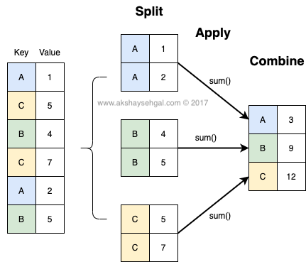
Before we can start writing code, let's explore the basics behind a groupby operation. The core concept behind any groupby operation is a three step process called Split-Apply-Combine.
Here is a diagram to make this more intuitive.
The syntax for using a groupby method in Pandas comprises of 2 parts. First is a grouper object and the second is the aggregator. The general structure looks like the following -
dataset.groupby(['grouping column(s)'])['output column(s)'].aggregation()
|____________________________________| |________________________________|
| |
grouper object (split) aggregation (apply & combine)
#Load dependencies
import pandas as pd
import numpy as np
import seaborn as sns
titanic = sns.load_dataset('titanic').dropna() #drop missing data
print(titanic.shape)
titanic.head()
(182, 15)
survived | pclass | sex | age | sibsp | parch | fare | embarked | class | who | adult_male | deck | embark_town | alive | alone | |
---|---|---|---|---|---|---|---|---|---|---|---|---|---|---|---|
1 | 1 | 1 | female | 38.0 | 1 | 0 | 71.2833 | C | First | woman | False | C | Cherbourg | yes | False |
3 | 1 | 1 | female | 35.0 | 1 | 0 | 53.1000 | S | First | woman | False | C | Southampton | yes | False |
6 | 0 | 1 | male | 54.0 | 0 | 0 | 51.8625 | S | First | man | True | E | Southampton | no | True |
10 | 1 | 3 | female | 4.0 | 1 | 1 | 16.7000 | S | Third | child | False | G | Southampton | yes | False |
11 | 1 | 1 | female | 58.0 | 0 | 0 | 26.5500 | S | First | woman | False | C | Southampton | yes | True |
Question: What is the total number of passengers from each class who survived?
#Step 1: Create grouper
grouper = titanic.groupby(['class'])
#Step 2: Filter column and apply aggregation
grouper['survived'].sum().reset_index()
class | survived | |
---|---|---|
0 | First | 106 |
1 | Second | 12 |
2 | Third | 5 |
You would usually do this in a single statement as the following:
titanic.groupby(['class'])['survived'].sum().reset_index()
class | survived | |
---|---|---|
0 | First | 106 |
1 | Second | 12 |
2 | Third | 5 |
Note: The
reset_index()
helps bring the grouping columns from index, back as a column in a dataframe.
Question: What was the average fare for passengers from each town?
titanic.groupby(['embark_town'])['fare'].mean().reset_index()
embark_town | fare | |
---|---|---|
0 | Cherbourg | 103.342503 |
1 | Queenstown | 90.000000 |
2 | Southampton | 64.922862 |
We can pass a list of features in the groupby()
to increase the levels for grouping the data as below.
Question: What was the average fare for male vs female passengers from each town?
titanic.groupby(['embark_town','sex'])['fare'].mean().reset_index()
embark_town | sex | fare | |
---|---|---|---|
0 | Cherbourg | female | 104.169609 |
1 | Cherbourg | male | 102.435355 |
2 | Queenstown | female | 90.000000 |
3 | Queenstown | male | 90.000000 |
4 | Southampton | female | 79.251179 |
5 | Southampton | male | 52.674461 |
Similarly, we can select a list of variables for which you need to apply the aggreate function.
Question: What was the average fare and age for male vs female passengers from each town?
titanic.groupby(['embark_town','sex'])[['fare', 'age']].mean().reset_index()
embark_town | sex | fare | age | |
---|---|---|---|---|
0 | Cherbourg | female | 104.169609 | 35.352941 |
1 | Cherbourg | male | 102.435355 | 39.774194 |
2 | Queenstown | female | 90.000000 | 33.000000 |
3 | Queenstown | male | 90.000000 | 44.000000 |
4 | Southampton | female | 79.251179 | 30.952830 |
5 | Southampton | male | 52.674461 | 37.595484 |
Before we go further and try other, more complex scenarios, let's try to understand the data structures we are working with, so that we can be much more creative with our approaches and get a deeper understanding on how they work.
You can imagine the pipeline of the above code to be as -
titanic.groupby(['embark_town'])
which splits data into the relevant groups'fare'
from each of those groupsmean()
on this column for each of the groups, combine and then return the aggregated datasetLet's see what the grouper object looks like for a better understanding.
grouper = titanic.groupby(['embark_town'])
#Print dtype for each of the elements in the grouper
[(type(k),type(g)) for k,g in grouper]
[(str, pandas.core.frame.DataFrame), (str, pandas.core.frame.DataFrame), (str, pandas.core.frame.DataFrame)]
So, this shows that if we try to iterate over the grouper object, its nothing but a tuple with the key and a dataframe.
Let's see what each of those is.
#Print shape for the dataframe groups
[(k,g.shape) for k,g in grouper]
[('Cherbourg', (65, 15)), ('Queenstown', (2, 15)), ('Southampton', (115, 15))]
The key for each of the tuples/groups is the value from the grouper column (in this case the embark_town
) and the value is just the complete dataframe filtered for that value! If we try to print one of the dataframe from this grouper, you can see that all the rows in this slice of data contain Queenstown
as the embark_town
, as shown below.
print(list(grouper)[1][0]) #print key
list(grouper)[1][1] #print dataframe
Queenstown
survived | pclass | sex | age | sibsp | parch | fare | embarked | class | who | adult_male | deck | embark_town | alive | alone | |
---|---|---|---|---|---|---|---|---|---|---|---|---|---|---|---|
245 | 0 | 1 | male | 44.0 | 2 | 0 | 90.0 | Q | First | man | True | C | Queenstown | no | False |
412 | 1 | 1 | female | 33.0 | 1 | 0 | 90.0 | Q | First | woman | False | C | Queenstown | yes | False |
Similarly, let's see how the grouper object looks like for multiple grouping features. The 'key' in this case is just a tuple with all the group combinations, which, after aggregation, gets set as the index of the final output.
grouper = titanic.groupby(['embark_town','sex'])
#Print dtype for each of the elements in the grouper
[(k,g.shape) for k,g in grouper]
[(('Cherbourg', 'female'), (34, 15)), (('Cherbourg', 'male'), (31, 15)), (('Queenstown', 'female'), (1, 15)), (('Queenstown', 'male'), (1, 15)), (('Southampton', 'female'), (53, 15)), (('Southampton', 'male'), (62, 15))]
#The grouping columns become the index after the groupby aggregation
titanic.groupby(['embark_town','sex'])['age'].mean()
embark_town sex Cherbourg female 35.352941 male 39.774194 Queenstown female 33.000000 male 44.000000 Southampton female 30.952830 male 37.595484 Name: age, dtype: float64
There are multiple ways of aggregating your grouper object.
apply()
or agg()
to write your own custom aggregators but Pandas makes it much easier by providing a ton of in-built aggregators such as sum()
or mean()
as we discussed in the above examples.Let's try to go through a few scenarios and explore how we can use these aggregations.
Pandas provides a ton of aggregation methods to quickly get the statistics you are looking for. Below are a few of the common ones that are use and more details on these can be found on the official pandas documentation.
Function | Description |
---|---|
mean( ) | Compute mean of groups |
median( ) | Compute median of groups |
mode( ) | Compute mode of groups |
sum( ) | Compute sum of group values |
prod( ) | Compute product of group values |
size( ) | Compute group sizes |
count( ) | Compute count of group |
std( ) | Standard deviation of groups |
var( ) | Compute variance of groups |
skew( ) | Compute skewness/3rd moment of groups |
kurt( ) | Compute kurtosis/4th moment of groups |
sem( ) | Standard error of the mean of groups |
mad( ) | Mean absolute deviation for each group |
describe( ) | Generates descriptive statistics |
first( ) | Compute first of group values |
last( ) | Compute last of group values |
nth( ) | Take nth value, or a subset if n is a list |
min( ) | Compute min of group values |
max( ) | Compute max of group values |
This is by far the most popular way of applying a custom function to a dataframe, or in this case, applying it on each of the dataframe slices for groups defined by the grouper. The behavior of the apply()
method with groupby is similar to the standard one.
You can apply it to each row (or column) of a dataframe input (if you have more than one column for aggregation) or to a series (if you have single column for aggregation). Within the function, you can actually either work directly with individual series or just write your own lambda function. Here are a few ways using the apply function.
Question: Get the unique set of ages for all each age category (who
column) from each town.
titanic.groupby(['embark_town', 'who'])['age'].apply(set).reset_index()
embark_town | who | age | |
---|---|---|---|
0 | Cherbourg | man | {17.0, 18.0, 23.0, 24.0, 25.0, 26.0, 27.0, 30.... |
1 | Cherbourg | woman | {16.0, 17.0, 18.0, 19.0, 21.0, 22.0, 23.0, 24.... |
2 | Queenstown | man | {44.0} |
3 | Queenstown | woman | {33.0} |
4 | Southampton | child | {0.92, 1.0, 2.0, 3.0, 4.0, 6.0, 11.0, 14.0, 15.0} |
5 | Southampton | man | {19.0, 21.0, 25.0, 27.0, 28.0, 29.0, 31.0, 32.... |
6 | Southampton | woman | {16.0, 17.0, 18.0, 19.0, 21.0, 22.0, 23.0, 24.... |
Question: Get the range (min - max) of ages for each age category (who
column) from each town.
titanic.groupby(['embark_town', 'who'])['age'].apply(lambda x: x.max()-x.min()).reset_index()
embark_town | who | age | |
---|---|---|---|
0 | Cherbourg | man | 54.00 |
1 | Cherbourg | woman | 44.00 |
2 | Queenstown | man | 0.00 |
3 | Queenstown | woman | 0.00 |
4 | Southampton | child | 14.08 |
5 | Southampton | man | 61.00 |
6 | Southampton | woman | 47.00 |
Question: Get the mean fare by age ratio for each age category (who
column) from each town.
titanic.groupby(['embark_town', 'who']).apply(lambda x: (x['fare']/x['age']).mean())
embark_town who Cherbourg man 3.146083 woman 3.614103 Queenstown man 2.045455 woman 2.727273 Southampton child 28.956893 man 1.410745 woman 2.593897 dtype: float64
Sooner or later, you would find it necessary to work with multiple aggregations over multiple columns at once. This is where agg()
method comes in. Here is a quick example of how you can use multiple in-built functions over multiple columns at once.
The general way to do this is to create a dictionary with the requirements and pass it to the agg()
function. There are a few ways to structure the dictionary -
##Single function per column
{
'column1': 'function1',
'column2': 'function2'
}
##Multiple functions per column
{
'column1': ['function1', 'function2'],
'column2': ['function3', 'function4']
}
Question: Get the mean of fare, AND median of age for each age category (who
column) from each town
#Define aggregations as a dictionary
g = {'fare':'mean',
'age':'median'
}
titanic.groupby(['embark_town', 'who']).agg(g).reset_index()
embark_town | who | fare | age | |
---|---|---|---|---|
0 | Cherbourg | man | 102.435355 | 36.0 |
1 | Cherbourg | woman | 104.169609 | 37.0 |
2 | Queenstown | man | 90.000000 | 44.0 |
3 | Queenstown | woman | 90.000000 | 33.0 |
4 | Southampton | child | 77.379485 | 4.0 |
5 | Southampton | man | 51.071515 | 40.0 |
6 | Southampton | woman | 77.686436 | 33.0 |
Question: Get the sum & mean of fare, AND median, min and max of age for each age category (who
column) from each town
#Define aggregations as a dictionary
g = {'fare':['sum', 'mean'],
'age':['median', 'min', 'max']
}
titanic.groupby(['embark_town', 'who']).agg(g).reset_index()
embark_town | who | fare | age | ||||
---|---|---|---|---|---|---|---|
sum | mean | median | min | max | |||
0 | Cherbourg | man | 3175.4960 | 102.435355 | 36.0 | 17.00 | 71.0 |
1 | Cherbourg | woman | 3541.7667 | 104.169609 | 37.0 | 16.00 | 60.0 |
2 | Queenstown | man | 90.0000 | 90.000000 | 44.0 | 44.00 | 44.0 |
3 | Queenstown | woman | 90.0000 | 90.000000 | 33.0 | 33.00 | 33.0 |
4 | Southampton | child | 1005.9333 | 77.379485 | 4.0 | 0.92 | 15.0 |
5 | Southampton | man | 2808.9333 | 51.071515 | 40.0 | 19.00 | 80.0 |
6 | Southampton | woman | 3651.2625 | 77.686436 | 33.0 | 16.00 | 63.0 |
As of Pandas >= 0.25, another way to define the agg
function is define the each column with ('column', 'function')
.
Let's demonstrate that with an example.
Question: Get the sum & mean of fare, AND min and max of age for each age category (who
column) from each town, but rename columns
#Define aggregations directly as columns and tuples
titanic.groupby(['embark_town', 'who']).agg(A=('fare', 'sum'),
B=('fare', 'mean'),
C=('age', 'min'),
D=('age', 'max')).reset_index()
embark_town | who | A | B | C | D | |
---|---|---|---|---|---|---|
0 | Cherbourg | man | 3175.4960 | 102.435355 | 17.00 | 71.0 |
1 | Cherbourg | woman | 3541.7667 | 104.169609 | 16.00 | 60.0 |
2 | Queenstown | man | 90.0000 | 90.000000 | 44.00 | 44.0 |
3 | Queenstown | woman | 90.0000 | 90.000000 | 33.00 | 33.0 |
4 | Southampton | child | 1005.9333 | 77.379485 | 0.92 | 15.0 |
5 | Southampton | man | 2808.9333 | 51.071515 | 19.00 | 80.0 |
6 | Southampton | woman | 3651.2625 | 77.686436 | 16.00 | 63.0 |
As you might think, just modifying the aggregate functions to include lambda functions is a way to create your own custom functions applied to specific columns. Here are a few examples.
#Define aggregations as a dictionary
g = {'fare':lambda x: x.sum(),
'age' :lambda x: x.max()
}
titanic.groupby(['embark_town', 'who']).agg(g).reset_index()
embark_town | who | fare | age | |
---|---|---|---|---|
0 | Cherbourg | man | 3175.4960 | 71.0 |
1 | Cherbourg | woman | 3541.7667 | 60.0 |
2 | Queenstown | man | 90.0000 | 44.0 |
3 | Queenstown | woman | 90.0000 | 33.0 |
4 | Southampton | child | 1005.9333 | 15.0 |
5 | Southampton | man | 2808.9333 | 80.0 |
6 | Southampton | woman | 3651.2625 | 63.0 |
Apart from just aggregating, you can use groupby to transform columns based on the grouper object. This requires using transform()
function and returns the same number of rows as the original dataset, but the functions are applied based on the grouping defined. Let's consider the following point.
Question: Create a new column that returns the average fare for the age group (who
column) the passenger belongs to.
titanic.groupby('who')['fare'].transform(lambda x: x.mean())
1 88.817429 3 88.817429 6 69.821026 10 77.379485 11 88.817429 ... 871 88.817429 872 69.821026 879 88.817429 887 88.817429 889 69.821026 Name: fare, Length: 182, dtype: float64
Notice that the output series is of the length of the original titanic dataframe, but contains only 3 unique values [88.8, 69.8, 77.3]
, one for each of the ['woman', 'man', 'child']
. This make the grouping object highly versatile in the way you would use it for data preprocessing.
Let's introduce a few advanced cases where you end up using groupby for data preprocessing.
The grouper object doesnt need to explicitly come from the dataframe. As long as the length of the grouper is the same as the number of rows in the dataframe, you can assign any grouper to groupby the rows by.
df = pd.DataFrame({'A':[1,2,3,4,8,10,12,13],
'B':[1,2,2,3,1,3,2,3]
})
#custom grouping
even_odd = ['even' if i%2==0 else 'odd' for i in df['A']]
df.groupby(even_odd)['B'].mean()
even 2.2 odd 2.0 Name: B, dtype: float64
Question: Get sum of the value
column of the given dataframe based on the sequentially occuring groups category
i.e, in [1,1,2,2,1,1]
the first group of 1's
should be a separate group than second set of 1's
.
We can solve this creating a custom grouper, by shifting the column value by 1 and comparing them with original. If not equal, it will swap the boolean value. Then we can take a
cumsum
over the boolean to get groups where the value changes consecutively. Here is the solution for a similar problem I solved on Stack Overflow.
df = pd.DataFrame({'A':[1,1,2,2,2,1,1,3,3], #<- column to group on
'B':[1,7,2,4,1,8,2,1,3] #<- column to aggregate
})
grouper = (df['A']!=df['A'].shift()).cumsum()
df.groupby(grouper).agg({'A':'mean','B':'sum'}).reset_index(drop=True)
A | B | |
---|---|---|
0 | 1 | 8 |
1 | 2 | 7 |
2 | 1 | 10 |
3 | 3 | 4 |
Question: A dataframe only contains rows for few dates for each id
. The goal is to re-index the dataframe for a fixed date range, but for each of the id
individually. Also, fill the missing data with 0 values.
Here we can create a custom reindex using
pandas.date_range
. Then, after setting the original date column as index, we can applypandas.DataFrame.reindex
along with groupby on theid
column to reindex with the new date range for group, while filling empty values as 0.
d = {'id': [11, 11, 11, 11, 13, 13, 13],
'date': ['2017-06-01','2017-06-03','2017-06-05','2017-06-06','2017-06-01','2017-06-02','2017-06-07'],
'value': [1, 7, 8, 2, 9, 2, 11]
}
df = pd.DataFrame(d)
df['date'] = pd.to_datetime(df['date'])
print("Input dataframe:")
df
Input dataframe:
id | date | value | |
---|---|---|---|
0 | 11 | 2017-06-01 | 1 |
1 | 11 | 2017-06-03 | 7 |
2 | 11 | 2017-06-05 | 8 |
3 | 11 | 2017-06-06 | 2 |
4 | 13 | 2017-06-01 | 9 |
5 | 13 | 2017-06-02 | 2 |
6 | 13 | 2017-06-07 | 11 |
#custom date range
idx = pd.date_range('2017-06-01','2017-06-07')
#set original date column as index
df.set_index('date', inplace=True)
#grouby and apply pd.DataFrame.reindex to apply new index and fill value as 0
df.groupby('id').apply(pd.DataFrame.reindex, idx, fill_value=0).drop('id',1).reset_index()
id | level_1 | value | |
---|---|---|---|
0 | 11 | 2017-06-01 | 1 |
1 | 11 | 2017-06-02 | 0 |
2 | 11 | 2017-06-03 | 7 |
3 | 11 | 2017-06-04 | 0 |
4 | 11 | 2017-06-05 | 8 |
5 | 11 | 2017-06-06 | 2 |
6 | 11 | 2017-06-07 | 0 |
7 | 13 | 2017-06-01 | 9 |
8 | 13 | 2017-06-02 | 2 |
9 | 13 | 2017-06-03 | 0 |
10 | 13 | 2017-06-04 | 0 |
11 | 13 | 2017-06-05 | 0 |
12 | 13 | 2017-06-06 | 0 |
13 | 13 | 2017-06-07 | 11 |
Here I discuss 3 ways that are popularly used to group data depending on the data structures and libraries you are already working with.
collections.defaultdict
numpy.split()
to group an arrayitertools.groupby()
Let's say we have a list of tuples with keys and values which we need to group.
data = list(zip(np.random.randint(0,4,(10,)), np.random.randint(0,100,(10,))))
print(data)
[(1, 41), (1, 30), (2, 70), (3, 82), (2, 68), (0, 18), (3, 97), (1, 37), (3, 8), (0, 51)]
A useful way of grouping data is to use defaultdict
. Defaultdict can store the grouping values as keys, and store the values as a list of values (or a custom function on them)
from collections import defaultdict
d = defaultdict(list)
for k,v in data:
d[k].append(v)
grouped_data = dict(d)
print(grouped_data)
{1: [41, 30, 37], 2: [70, 68], 3: [82, 97, 8], 0: [18, 51]}
Another way of splitting an array into a list of sub-arrays based on a grouping key is by using np.split
along with the indexes for each group returned by np.unique
. Only important thing is, the arrays needs to be sorted explicitly.
import numpy as np
#sorted numpy array (sorted by the grouping column)
a = np.array(data)
a = a[np.argsort(a[:, 0])]
#Take the index positions for the unique values using return_index
#and start from the second one to split the data
groups = np.split(a[:,1], np.unique(a[:,0], return_index=True)[1][1:])
print(groups)
[array([18, 51]), array([41, 30, 37]), array([70, 68]), array([82, 97, 8])]
import itertools
items = sorted(data, key=lambda x:x[0])
grouper = itertools.groupby(items, key=lambda x:x[0])
groups = [list(g) for k, g in grouper]
groups
[[(0, 18), (0, 51)], [(1, 41), (1, 30), (1, 37)], [(2, 70), (2, 68)], [(3, 82), (3, 97), (3, 8)]]