python machinelearning naivebayes classification
© Copyright 2019, Akshay Sehgal | 13th Jan 22
Prerequisites: Basic understanding of Python & Scikit-learn library
Naive Bayes is a supervised classification algorithm which belongs to the family of "Probabilistic Classifiers". As the name suggests, it is uses Bayes' theorem at its core with a 'naive' assumption.
The algorithm is widely used for simple classification problems and works well with text data in a bag of words form. Infact, it was most popularized by its use as a spam email classifier by google. To this date, its widely used as a benchmarking model by data scientists in hackatons on kaggle.
Before we get into the crux of the algorithm, its important to know what bayes rule is.
You can get a great intuitive sense about conditional probability from lectures of Prof John Tsitsiklis (MITOpenCourseware).
"You know something about the world, and based on what you know, you setup a probability model and you write down probabilities about the different outcomes. Then someone gives you some new information, which changes your beliefs and thus changes the probabilities of your outcomes."
In a simple sense, bayes' theorem talks about the 'new' probabilities of an experiment given that an event has occured.
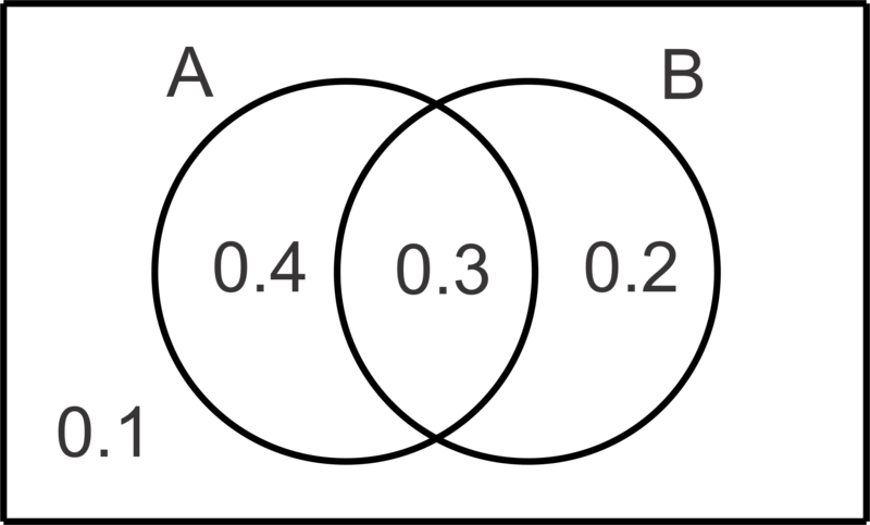
Let's say you have a sample space the probabilities for different events are given as below -
Now let's say someone tells you that B has occured. The area outside the circle that represents B is now meaningless since the new sample space is now B. This means, we need to revise the probabilities that have been assiged to the spaces inside B.
Now someone asks you, what is the probability that A occurs, given that B has occured. Since B has occured and the new sample space is now B, the area that was initially represented by $P(A \cap B)$ is now the $P(A \mid B)$. But the probability now has to be recalculated.
What is the probability of this new section? Well, we can just use simple ratios for solving this.
$$ P (A \mid B) = {P(A \cap B) \over P(B)} = {0.3 \over (0.3+0.2)}$$Now, the whole exercise we did above can also be done for when A has occured. Meaning that we can use symmetry to show -
$$ P (B \mid A) = {P(A \cap B) \over P(A)}$$Using the two symmetric equations and replacing $P(A \cap B)$, we can write the famous equation -
$$ P (A \mid B) = {P (B \mid A) \times P(A) \over P(B)}$$Now, let's see an 'expanded' version of this definition which is more relevant to data science. We want to know what is the probability of $y$ given that $x_1, x_2, ... , x_n$ have occured (where $x_i$ are different features and y is the class label we want to predict). This is given by -
$$P(y \mid x_1, x_2, ... , x_n) = {P(x_1, x_2, ... , x_n \mid y) \times P(y) \over P(x_1, x_2, ... , x_n)}$$Here comes the Naive assumption of conditional independence. The assumption is that all the features $x_1, x_2 ..., x_n$ are independent. This means that $P(A,B) = P(A).P(B)$. Applying this to the above equation we get -
$$P(y \mid x_1, x_2, ... , x_n) = {P(x_1 \mid y).P(x_2 \mid y)... P(x_n \mid y).P(y) \over P(x_1).P(x_2)...P(x_n)}$$Using proper convention -
$$P(y \mid x_1, x_2, ... , x_n) = {P(y)\prod_{i=1}^{n} P(x_i \mid y) \over \prod_{i=1}^{n} P(x_i)}$$Since the denominator is constant, we can write the equation as -
$$P(y \mid x_1, x_2, ... , x_n) \propto P(y)\prod_{i=1}^{n} P(x_i \mid y)$$In order to turn this into a classifier, we need to pick up the one with the max probability. This can be expressed as -
$$y = argmax_y(P(y)\prod_{i=1}^{n} P(x_i \mid y))$$The last step is known as Maximum A Posteriori decision rule.
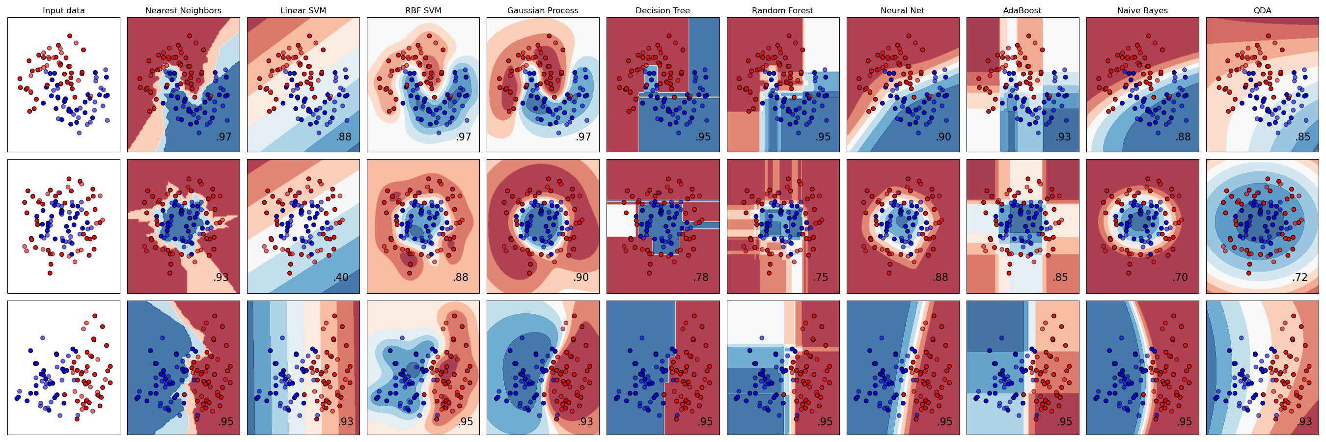
When working with different algorithms, its important to undertand where a particular algorithm will work and where it may not. For this, I have always found a 2 dimensional example of decision boundaries quite useful from an intuitive point of view, since the core 'nature' of the classifier retains itself in higher dimensional spaces as well. The objective is to separate the blue from the red points. The decision boundary with the confidence is plotted.
Notice below (image from sklearn documentation), the naive bayes classifier is capable of fitting smooth continous decision boundaries, but fails when the data needs a high degree polynomial.
Now, when you actually plan on implementing this, you will notice there are multiple classifiers available that can be used for a naive bayes model. The three classifiers behave almost the same way, however with minor differences and assumptions. The above equation calculates $P(x_i \mid y)$ in a straight forward way for features with discrete values, but what if the features are continous variables. Clearly, this will need you to 'assume' the nature of the distribution since unlike discrete valued features, where you could just sum up the number of times a discrete value occured along with the specific y class label. In this case we can use classifiers such as GaussianNB.
Simply put, by choosing different classifiers, you get to choose the assumptions regarding the nature of distributions of $P(x_i \mid y)$. More about these classifiers in later sections.
Lets do a quick implementation of Naive Bayes. This is how you would actually implement it when working with data. The focus will be on the algorithm rather than data preprocessing for now. For this example, I will select the iris data which is available as part of the sklearn datasets API.
# Loading the dependencies for the model
import pandas as pd
import numpy as np
from sklearn.datasets import load_iris
from sklearn.model_selection import train_test_split
from sklearn.naive_bayes import GaussianNB
import math
# Loading the iris data into X, y. Each dataset will have its own way of doing this.
iris = load_iris()
X = iris.data
y = iris.target
y_labels = iris.target_names
X_labels = iris.feature_names
#4 features, 150 samples, 3 target values to predict
print("Column names - ",X_labels)
print("Shape of X - ",X.shape)
print("Target values - ",y_labels)
Column names -  ['sepal length (cm)', 'sepal width (cm)', 'petal length (cm)', 'petal width (cm)']
Shape of X -  (150, 4)
Target values -  ['setosa' 'versicolor' 'virginica']
#Separating test and train data for model evaluation
X_train, X_test, y_train, y_test = train_test_split(X,y, test_size = 0.2)
#Instantiate the classifier and fit it to training data
nb = GaussianNB()
nb.fit(X_train, y_train)
GaussianNB(priors=None, var_smoothing=1e-09)
#Evaluation of the model using test data
nb.score(X_test, y_test)
0.9333333333333333
# Model's prediction when sepal_len = 5.8, sepal_wid = 2.2, petal_len = 4.2, petal_wid = 0.4
nb.predict([[5.8,2.2,4.2,0.4]])
array([1])
The value 1 corresponds to versicolor, as seen by the y_labels (0 represents setosa). This is a straightforward sklearn workflow and should be quite familiar if you have implemented any model with sklearn before.
This section we are going to implement the different classifiers from scratch, making sure we actually show what's happening behind the scene. Also, since I am not a big fan of for loops, I will try to give a vectorized implementation of the model, as much as possible.
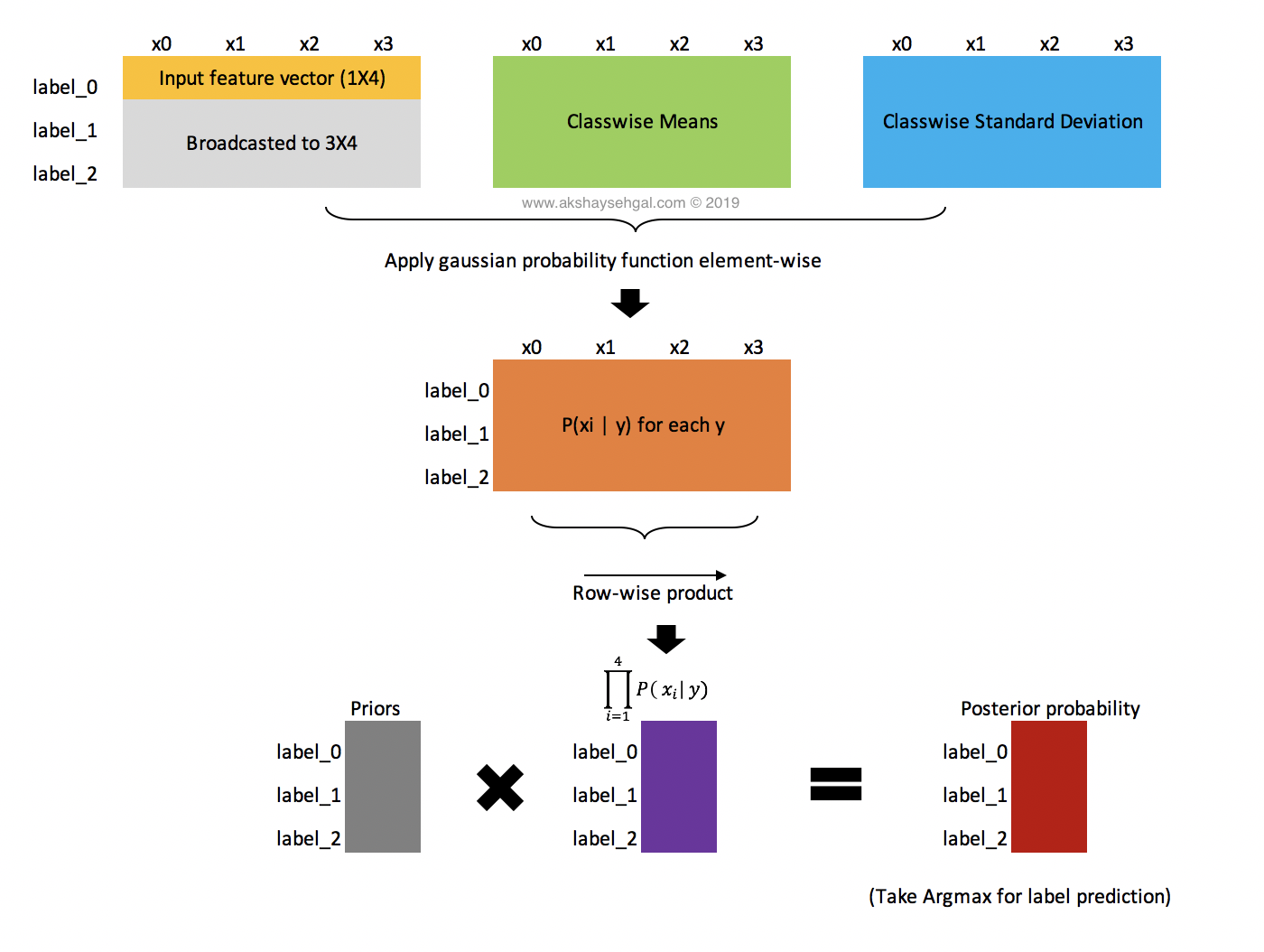
When your features are continous in nature, you assume that they are conditionally independent and that the data associated with each class is normally distributed. To calculate the $P(x_i \mid y)$ values, we segment the data by the class, compute mean, variance and then derive the probability distribution as below.
$$P(x_i \mid y) = {1 \over \sqrt{2 \pi \sigma^2_y}}exp \Bigg(-{(x_i - \mu_y)^2 \over 2 \sigma^2_y} \Bigg)$$The first step is to calculate the summary statistics. For gaussian classifier, we need the class-wise mean and standard deviation and we need the class priors, which is nothing but the class probability in the entire data. With these 3, we should be able to predict which class a particular sample belongs to. Following is a diagram which shows the vectorized computation of the gaussian classifier in a graphical representation.
#Putting all the data into a dataframe
df = pd.DataFrame(X, columns=X_labels)
df['class'] = y
df.head()
| sepal length (cm) | sepal width (cm) | petal length (cm) | petal width (cm) | class | |
|---|---|---|---|---|---|
| 0 | 5.1 | 3.5 | 1.4 | 0.2 | 0 |
| 1 | 4.9 | 3.0 | 1.4 | 0.2 | 0 |
| 2 | 4.7 | 3.2 | 1.3 | 0.2 | 0 |
| 3 | 4.6 | 3.1 | 1.5 | 0.2 | 0 |
| 4 | 5.0 | 3.6 | 1.4 | 0.2 | 0 |
#Calculating class priors (simply the probability of class labels)
priors = np.unique(y, return_counts=True)[1] / len(y)
priors
array([0.33333333, 0.33333333, 0.33333333])
#Class wise mean for each feature
classwise_means = df.groupby(['class']).mean().reset_index()
classwise_means
| class | sepal length (cm) | sepal width (cm) | petal length (cm) | petal width (cm) | |
|---|---|---|---|---|---|
| 0 | 0 | 5.006 | 3.428 | 1.462 | 0.246 |
| 1 | 1 | 5.936 | 2.770 | 4.260 | 1.326 |
| 2 | 2 | 6.588 | 2.974 | 5.552 | 2.026 |
#Class wise mean for each feature
classwise_std = df.groupby(['class']).std().reset_index()
classwise_std
| class | sepal length (cm) | sepal width (cm) | petal length (cm) | petal width (cm) | |
|---|---|---|---|---|---|
| 0 | 0 | 0.352490 | 0.379064 | 0.173664 | 0.105386 |
| 1 | 1 | 0.516171 | 0.313798 | 0.469911 | 0.197753 |
| 2 | 2 | 0.635880 | 0.322497 | 0.551895 | 0.274650 |
# Gaussian probability function vectorized to work on multidimensional arrays with broadcasting
def pdf(x, mean, sd):
    return (1 / np.sqrt(2*np.pi*sd**2)) * np.exp(-1*((x-mean)**2/(2*sd**2)))

vectorized_pdf = np.vectorize(pdf)
#Converting everything to numpy arrays
mean_array = np.array(classwise_means.iloc[:,1:])
std_array = np.array(classwise_std.iloc[:,1:])

#Sample is the feature vector, whose label needs to be predicted
sample = [5.1, 3.5, 1.4, 0.2]
#Element wise application of the pdf(x,mean,std) function on broadcasted arrays
elementwise_pdf = vectorized_pdf(sample, mean_array, std_array)
elementwise_pdf
array([[1.09224777e+00, 1.03362481e+00, 2.15537744e+00, 3.44157106e+00],
       [2.08211139e-01, 8.49365434e-02, 7.67726912e-09, 1.83893298e-07],
       [4.05935486e-02, 3.27130259e-01, 3.70613589e-13, 3.66254229e-10]])
#Rowwise product of the above matrix
rowwise_product = np.product(elementwise_pdf,axis=1)
rowwise_product
array([8.37460175e+00, 2.49672786e-17, 1.80252677e-24])
#Elementwise multiplication with corresponding class probabilities (priors)
multiply_priors = np.multiply(priors,rowwise_product)
multiply_priors
array([2.79153392e+00, 8.32242620e-18, 6.00842257e-25])
#Argmax to predict class label
prediction = np.argmax(multiply_priors)
prediction
0
The 0 here means first class 'setosa'.
Few interesting notes based on this calculation -
Multinomial classifier is a bit more complex but is the usual choice for text based data. Here you assume that your data is distributed multinomially. Multinomial distribution is a generalized case of binomial, bernoulli and categorical distributions depending on the number of trials (n) and the number of outcomes (k). If there are only 2 possible outcomes (k=2) and multiple trials (n>1) then your multinomial distribution becomes a binomial distribution.
Lets say you have a few sentences with labels -
Lets say you are asked to classify the sentence "Great smartphone". What you are trying to do is to just find the probability of the words "Great" and "Smartphone" to occur with the label Positive/Negative. Based on the product of the probabilities of the 2 words (remember the 'naive' assumption) you calculate which has a higher product of probabilities and then predict that as the corresponding label. This is done by simply calculating $N_w / N$ where $N_w$ is the number of times the word occurs with the label, and N is the total number of words that occur with the given label.
Here comes the issue while doing this. If the word isn't used in the traning data (like in this case "Smartphone"), the value of the product of probabilities will become 0. How do we solve this? We use a techinque called additive smoothing (laplace smoothing) which just adds some stuff to the numerator and denominator. $P(x_i \mid y)$ is the probability $\theta_i$ of $i$ appearing in a sample belonging to $y$.
$$ \hat\theta_i = {N_w + \alpha \over N + \alpha d} $$Here $\alpha$ is set to 1 incase of laplace smoothing, while $\alpha$ is set > 1 for Lidstone smoothing. $N_w$ is the number of times the word occurs with that label, N is the number of words in vocabulary which occur with that label, and d is the total size of the vocabulary.
Note that for the implementation I will only show the case where we use count vectorizer but for improving the model, it is important to leverage various techiniques such as stopword removal, lemmitization, tfidf vectorizer etc. We will start with creating a small text dataset with 2 labels.
from sklearn.feature_extraction.text import CountVectorizer
#Defining the training data
documents = ['quite happy with it',
             'bad device',
             'great job with the features',
             'bad experience',
             'horrible device',
             'very happy with the product']

classes = ['positive','negative','positive','negative','negative','positive']
#Fitting the count vectorizer to get word representation for each sentence
cnt = CountVectorizer()
cnt_matrix = cnt.fit_transform(documents).todense()
cnt_matrix.shape
(6, 14)
#Creating a dataframe to calculate summary statistics later
training_data = pd.DataFrame(cnt_matrix,
                                index = documents,
                                columns=cnt.get_feature_names())
training_data['Class'] = classes
training_data
| bad | device | experience | features | great | happy | horrible | it | job | product | quite | the | very | with | Class | |
|---|---|---|---|---|---|---|---|---|---|---|---|---|---|---|---|
| quite happy with it | 0 | 0 | 0 | 0 | 0 | 1 | 0 | 1 | 0 | 0 | 1 | 0 | 0 | 1 | positive |
| bad device | 1 | 1 | 0 | 0 | 0 | 0 | 0 | 0 | 0 | 0 | 0 | 0 | 0 | 0 | negative |
| great job with the features | 0 | 0 | 0 | 1 | 1 | 0 | 0 | 0 | 1 | 0 | 0 | 1 | 0 | 1 | positive |
| bad experience | 1 | 0 | 1 | 0 | 0 | 0 | 0 | 0 | 0 | 0 | 0 | 0 | 0 | 0 | negative |
| horrible device | 0 | 1 | 0 | 0 | 0 | 0 | 1 | 0 | 0 | 0 | 0 | 0 | 0 | 0 | negative |
| very happy with the product | 0 | 0 | 0 | 0 | 0 | 1 | 0 | 0 | 0 | 1 | 0 | 1 | 1 | 1 | positive |
#Calculating label probability (priors)
label_proba = np.unique(classes, return_counts=True)[1]/len(classes)
label_proba
array([0.5, 0.5])
#Calculating word frequency for each word in training data (label-wise)

## 0 = negative, 1 = positive
Nc = training_data.groupby(['Class']).sum().reset_index('Class').drop('Class',axis=1)
Nc
| bad | device | experience | features | great | happy | horrible | it | job | product | quite | the | very | with | |
|---|---|---|---|---|---|---|---|---|---|---|---|---|---|---|
| 0 | 2 | 2 | 1 | 0 | 0 | 0 | 1 | 0 | 0 | 0 | 0 | 0 | 0 | 0 |
| 1 | 0 | 0 | 0 | 1 | 1 | 2 | 0 | 1 | 1 | 1 | 1 | 2 | 1 | 3 |
# Calculating N which is the total number of word occurances associated with each label
N = np.sum(np.array(Nc),axis=1)
N
array([ 6, 14], dtype=int64)
#Calculating length of vocabulary
d = len(cnt.get_feature_names())
d
14
#Setting value of the laplace smoothing factor alpha
a = 1
#Getting theta for a single input word
def get_thetas(word):
    try:
        return (np.array(Nc[word]) + a) / (N+d)
    except:
        return (np.array([0]*len(Nc)) + a) / (N+d)

get_thetas('happy')
array([0.05 , 0.10714286])
#The sentence for which label needs to be predicted (word tokenized from start)
sample = ['happy', 'with', 'the', 'product']
# Calculating product of the probabilities for each word (label-wise)
probability_product = np.product(np.array([list(get_thetas(i)) for i in sample]), axis=0)
probability_product
array([6.25000000e-06, 1.17138692e-04])
#Prediction of label using argmax after multiplying the thetas with label probabilities (priors)
np.argmax(np.multiply(label_proba, probability_product))
1
The 1 here represents 'positive' label.
Quite clearly, the first thing that comes to mind is that if we replace the count vectorizer with tfidf vectorizer, the words that are not so important at representing a label will get lesser weights, while improving the weights for words which actually represent the labels. In this case, words like device, experience etc each contribute to either positive or negative labels respectively.
Similarly, removing stopwords and lemmatizing words will have even more impact on the accuracy of the model.